The very first step in the reception of the signals is the integration over the FRI interval by the device driver. This step can be expressed in pseudo-C-code like this:
    #define MODULUS  (SAMPLE_RATE * 2 * GRI_INTERVAL)
    int h[MODULUS];
    int idx;

    i = 0;
    while(1) {
		a = get_sample_from_adc();
		h[i] += (a - h[i]) / DECAY;
		i++;
		if (i >= MODULUS)
			i = 0;
    }
This is a running, exponential average of the signal in each sampling interval over the FRI period of the LORAN-C signal. But how does that look to other radio signals and background noise ?
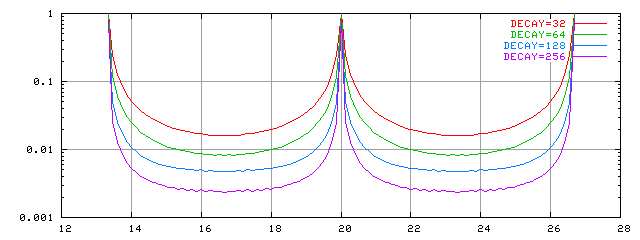
Another way to view the above is as a "comb-filter". "Comb-filters" are named that way because the frequency response looks very much like a personal hair-care tool: An endless sequence of equidistant peaks.
For the GRI=74990usec chain, the peaks are located 1 / (2 * 74990usec) = 6.66755... Hz apart. The plot below shows two periods of this filter, for various values of the "DECAY" parameter.
Since the LORAN-C signal we are after has a period of 1 / 74990usec = 13.335... Hz it will not be attenuated by the filter at all.
Figuring out what this filter does to other signals is somewhat tricky, so I built a small simulation to find out, the results are in the table below.
For random noise the results answer is pretty simple and good attenuation is obtained for even moderate values of DECAY.
Very few normal CW ("Continuous Wave") radio signals have bandwidths as narrow as the peaks and valleys of such a filter, so the overall effect of the GRI/FRI integration on those will be to attenuate them with the average value over one period of the filter. The simulation shows this to be is about 6dB less attenuation than for random noise, which makes sense when the periodic nature of CW signals is taken into account. Since most of these signals has a modulation, the real number will be in somewhere between these two extreemes.
| CW | Noise | |||
| DECAY | Ratio | dB | Ratio | dB |
| 32 | .070 | -3 | .33 | -9 |
| 64 | .048 | -6 | .25 | -12 |
| 128 | .032 | -9 | .17 | -15 |
| 256 | .028 | -12 | .11 | -18 |
As can be seen, larger DECAY factor is better, but two very real factors put upper limits on the usable DECAY factor: The stability of the timebase and rounding errors. So far I have used DECAY=128, but some experimentation is clearly called for.